[AI] 2-3. 優化器 Optimizer

在神經網路中，每個神經層都通過以下的方式進行資料轉換
output = relu(dot(W, input) + b)
W 和 b 為該層的屬性張量，統稱為該層的權重(weights) 或可訓練參數(trainable parameters)，分別為 內核(kernel) 屬性和 偏值(bias) 屬性。
我們的目標是要透過訓練(training) 來進行權重的微調，進而得到最小的損失值。
參數調大或調小，可能會對應到「損失值變大」或「損失值變小」兩種可能(如果兩者皆變小，稱為 saddle point，兩者皆變大，可能為 local minium)。
但如果透過兩個方向的正向傳播來檢查微調的方向，效率很低，於是科學家引入了梯度下降法。

梯度下降法(gradient descent)

張量運算的導數稱為梯度(gradient)。
- 純量函數的導數相當於在函數曲線上找某一點的斜率。
- 張量函數上求梯度，相當於在函數描繪的多維曲面上求曲率。

y_pred = dot(W, x)
loss_value = loss(y_pred, y_true)

假設只考慮 W 為變數，我們可以將 loss_value 視為 W 的函數。

loss_value = loss(dot(W, x), y_true) = f(W)

假設 W 的當前值為 W0，那麼函數 f 在 W0 這點的導數就是

$f’(W)=\frac{d\text{(loss\_value)}}{d\text{W}}|\text{W}_0$ 我們將上式寫成

g = grad(loss_value, W0)

代表了在 W0 附近，loss_value = f(W) 的梯度最陡方向之張量，我們可以透過往往「斜率反方向」移動來降低 f(W)。

if g > 0:
    W' = W0 - dW
elif: g < 0:
    W' = W0 + dW

我們將 g 直接代入式子，並引入 $\eta$ (eta) 的概念， $\eta$ 可以想成是每次移動的步伐大小。

W' = W0 - g * eta

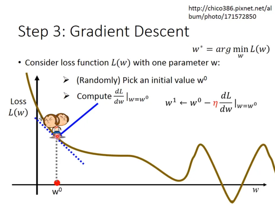
藉由不斷迭代，直到最後平緩，代表移到動 local minimum。但這個 local minimum 不一定是 global minimum，所以後面會加入其它方法來避免被 trap 在 local minimum。
以下是李宏毅老師的圖解，我覺得很生動，可以幫助理解。
圖解

隨機梯度下降

從上述的推導，其實我們可以設想，如何快速取得最小的損失值，方法是找出所有導數為 0 的點，再對這些點進行檢查，便可求出 global minimum。
然後對實際的神經網路而言，參數不會只有 2~3 個，可能會有上千萬個，故要求這樣的方程式解並非容易的事。
於是我們可以透過 小批次隨機梯度下降(mini-batch stochastic gradient descent, mini-batch SGD) 來進行
1. 取出一批次的訓練樣本 x 和對應的目標 y_true(也是標籤(label))
2. 以 x 為輸出資料，運行神經網路獲得預測值 y_pred。此步驟稱為正向傳播(forward pass)
3. 計算神經網路的批次損失值。
4. 計算損失值相對於神經網路權重的梯度。
5. 將參數稍微向梯度的反方向移動，從而降低一些批次損失值。此步驟稱為反向傳播(back propagation) $W’ = W - \eta \times \frac{dL}{dW}$ 其中 $\eta$ 為學習率(learning rate)，為純量因子，可用來調整梯度下降的速度。
  - 學習率太大太小都可能產生問題
    - 學習率太大可能會略過真正的最小值
    - 學習率太小可能會困在區域最小值
批次的量(batch size)
- 一次將所有的資料全用上，稱為整批 SGD(batch gradient descent)，好處是每次參數值更新會更準確，但是也會提升時間複雜度。
- 為了在「準確度」與「複雜度」取一個 tradeoff，通常會使用合理大小的小批次資料進行計算。

SGD 的變體

在計算下一次權重的更新量，可以考慮先前的取重更新量來做調整，而非僅僅根據梯度的當前值。常見的變體包含：

momemtum

past_velocity = 0.
momemtum = 0.1  # 固定的動量因數
while loss > 0.01:
    w, loss, gradient = get_current_parameters()
    velocity = past_velocity * momemtum - learning_rate * gradient
    w = w + momemtum * velocity - learning_rate * gradient
    past_velocity = velocity
    update_parameter(w)

Adagrad
RMSProp

反向傳播演算法(Backpropagation)

前面介紹的函數是簡單函式，可以很簡單地算出導數(梯度)，但在實際情況下，我們需要能夠處理複雜函數的梯度。

連鎖律(Chain Rule)

反向傳播是借助簡單運算(eg. 加法、relu或是張量積)的導數，進而得出這算簡單運算的複雜組合的梯度。
舉例而言，如下圖，我們使用了兩個密集層做轉換，

$\boxed{ \begin{array}{ccccccc} && \text{輸入資料 X} & \\ && \downarrow & \\ \boxed{\text{權重’}} & \rightarrow & \boxed{\text{層(資料轉換)}} & \red{\text{relu(W1,b1)}}\\ \uparrow && \downarrow & \\ \boxed{\text{權重’}} & \rightarrow & \boxed{\text{層(資料轉換)}} & \red{\text{softmax(W1,b2)}}\\ && \downarrow & \\ \uparrow && \boxed{\text{預測 Y’}}\rightarrow & \boxed{\text{損失函數}} & \leftarrow & \boxed{\text{標準答案 Y}} \\ &&& \downarrow & \\ \boxed{\text{優化器}} && \leftarrow & \boxed{\text{損失分數}} \end{array} }$

我們可以把函式表運成：

y1 = relu(dot(W1, X)+b1)
y2 = softmax(dot(W2, y1)+b2)
loss_value = loss(y_true, y2)

或

loss_value = loss(y_true, softmax(dot(W2, relu(dot(W1, X)+b1))+b2))

我們可以透過連鎖律求得連鎖函數的導數：假設有 $f$ , $g$ 兩個函數，它們的複合函數 $fg$ 有著 $fg(x)=f(g(x))$ 的特性。

def fg(x):
    x1 = g(x)
    y = f(x1)
    return y

根據連鎖律 $y=f(x_1,x_2,x_3…x_n),\frac{d\text{y}}{d\text{x}}=\red{\frac{d\text{y}}{d\text{x}_1}\times\frac{d\text{x}_1}{d\text{x}_2}\times\frac{d\text{x}_2}{d\text{x}_3}\times…\times\frac{d\text{x}_n}{d\text{x}}}$ 換言之，我們只需要求出 $\frac{d\text{y}}{d\text{x}_1}\times\frac{d\text{x}_1}{d\text{x}_2}\times\frac{d\text{x}_2}{d\text{x}_3}\times…\times\frac{d\text{x}_n}{d\text{x}}$ 就可以知道找出複合函數 $y$ 的導數了。

詳述

前向傳播
對於一個神經元，輸入值

\text{x}

通過權重

\text{w}

和偏置

\text{b}

進行線性組合，然後通過激活函數

\text{relu}

：

\text{z}=\text{wx+b}

\text{y}=\text{relu(z)}

損失函數
假設使用均方誤差(MSE)作為損失函數： $L = \frac{1}{2}(\text{y} - \text{y}_\text{true})^2$

反向傳播
使用連鎖律計算損失函數對權重的偏導數： $\frac{\partial L}{\partial \text{w}} = \frac{\partial L}{\partial \text{y}} \cdot \frac{\partial \text{y}}{\partial \text{z}} \cdot \frac{\partial \text{z}}{\partial \text{w}}$ 分解每一項：

$\frac{\partial L}{\partial \text{y}} = (\text{y} - \text{y}_\text{true})$ $\frac{\partial \text{y}}{\partial \text{z}} = \text{relu}’(\text{z})$ $\frac{\partial \text{z}}{\partial \text{w}} = \text{x}$

因此： $\frac{\partial L}{\partial \text{w}} = (\text{y} - \text{y}_\text{true}) \cdot \text{relu}’(\text{z}) \cdot \text{x}$

權重更新
使用梯度下降更新權重： $\text{w’} = \text{w} - \eta \frac{\partial L}{\partial \text{w}}$

思考正向傳播時，我們計算的順序是 $\text{z}\rightarrow\text{y}\rightarrow L$
而在推導梯度時，我們計算的順序是，剛好是反向過來計算的，故這個過程稱作「反向傳播」 $\frac{\partial L}{\partial \text{y}}\rightarrow\frac{\partial \text{y}}{\partial \text{z}}\rightarrow\frac{\partial \text{z}}{\partial \text{w}}$

如今我們在現代框架中，已經可以透過自動微分來實作神經網路，如 TensorFlow 的 Gradient Tape。故我們可以只專注在「正向傳播」的過程。

TensorFlow 的 Gradient Tape

透過 TensorFlow 的 Gradient Tape 函式，可以快速的取得微分值：

其中 tf.Variable 是一個變數物件，它可以是任意階的張量
範例：

import tensorflow as tf
x = tf.Variable(0.)
with tf.GradientTape() as tape:
  y = 2 * x + 3

grad = tape.gradient(y, x)
grad

>>> <tf.Tensor: shape=(), dtype=float32, numpy=2.0>

實作一個簡單的模型

Dense Layer

作用是將 input 與 W 做點積，與 b 相加，再輸入激活函數 f
相當於 y = f(wx+b)

import tensorflow as tf

class NaiveDense:
  def __init__(self, input_size, output_size, activation):
    self.activation = activation
    w_shape = (input_size, output_size)
    w_initial_value = tf.random.uniform(w_shape, minval = 0, maxval = 0.1)
    self.W = tf.Variable(w_initial_value)
    b_shape = (output_size, )
    b_initial_value = tf.zeros(b_shape)
    self.b = tf.Variable(b_initial_value)

  def __call__(self, inputs):
    return self.activation(tf.matmul(inputs, self.W) + self.b)

  @property
  def weights(self):
    return [self.W, self.b]

Sequential

Sequential 用來定義層與層之間連接的方式
在次簡單的用「依序」的方式進行正向傳播

class NaiveSequential:
  def __init__(self, layers):
    self.layers = layers

  def __call__(self, inputs):
    x = inputs
    for layer in self.layers:
      x = layer(x)
    return x

  @property
  def weights(self):
    weights = []
    for layer in self.layers:
      weights += layer.weights
    return weights

Build Model

通過上面兩個實作，便可以簡單建立一個 Keras 雙層模型：

model = NaiveSequential([
    NaiveDense(input_size=28*28, output_size=512, activation=tf.nn.relu),
    NaiveDense(input_size=512, output_size=10, activation=tf.nn.softmax)
])

Batch Generator

我們需要用「小批次」的方式來迭代，能更有效率的訓練資料：

import math
class BatchGeneartor:
  def __init__(self, images, labels, batch_size=128):
    assert len(images) == len(labels)
    self.index = 0
    self.images = images
    self.labels = labels
    self.batch_size = batch_size
    self.num_batches = math.ceil(len(images) / batch_size)

  def next(self):
    images = self.images[self.index : self.index + self.batch_size]
    labels = self.labels[self.index : self.index + self.batch_size]
    self.index += self.batch_size
    return images, labels

Update Weights

接下來我要透過 $\text{w’}=\text{w}-\eta\frac{dL}{d\text{W}}$ 來更新 W：

def update_weights(gradients, weights, learning_rate=1e-3):
  for g, w in zip(gradients, weights):
    w.assign_sub(g * learning_rate)

事實上我們不會這樣更新權重，我們可以借用 keras 的 optimizers

from tensorflow.keras import optimizers
optimizer = optimizers.SGD(learning_rate=1e-3)
def update_weights(gradients, weights):
  optimizer.apply_gradients(zip(gradients, weights))

Training

有了以上的工具，我們就可以進行訓練了

def one_training_step(model, images_batch, labels_batch):
  with tf.GradientTape() as tape:
    # y' = f(wx+b)
    predictions = model(images_batch)    
    # loss[] = y' - y_true
    per_sample_losses = (tf.keras.losses.sparse_categorical_crossentropy   (labels_batch, predictions))    
    # avg_loss = loss
    average_loss = tf.reduce_mean(per_sample_losses)[] / batch_size
    # g = grad(L, w)
    gradients = tape.gradient(average_loss, model.weights)  
    # w' = w-ηg
    update_weights(gradients, model.weights)
    return average_loss

def fit(model, images, labels, epochs, batch_size=128):
  for epoch_counter in range(epochs):
    print(f"Epoch {epoch_counter}")
    batch_generator = BatchGeneartor(images, labels)
    for batch_counter in range(batch_generator.num_batches):
      images_batch, labels_batch = batch_generator.next()
      loss = one_training_step(model, images_batch, labels_batch)
      if batch_counter % 100 == 0:
        print(f"loss at batch {batch_counter}: {loss:.2f}")

執行

from tensorflow.keras.datasets import mnist
(train_images, train_labels),(test_images, test_labels) = mnist.load_data()

train_images = train_images.reshape((60000, 28*28))
train_images = train_images.astype("float32") / 255
test_images = test_images.reshape((10000, 28*28))
test_images = test_images.astype("float32") / 255

fit(model, train_images, train_labels, epochs=10, batch_size=128)

Evaluation

最後我們再投入 test_images 來評估我們 training 的結果

import numpy as np

predictions = model(test_images)
predictions = predictions.numpy()

predicted_labels = np.argmax(predictions, axis=1)
matches = predicted_labels == test_labels
print(f"accuracy: {matches.mean():.2f}")

梯度下降法(gradient descent)#

隨機梯度下降#

反向傳播演算法(Backpropagation)#

連鎖律(Chain Rule)#

TensorFlow 的 Gradient Tape#

實作一個簡單的模型#

Dense Layer#

Sequential#

Build Model#

Batch Generator#

Update Weights#

Training#

Evaluation#