[AI] 二元分類問題

1. 認識 IMDB 資料集

• 透過 tensorflow 引入資料集
  • 參數
    • path: 資料的快取位置（相對於 ~/.keras/dataset）。
    • num_words: 整數或 None。單詞按其出現頻率（在訓練集中）進行排序，並且僅保留 num_words 個最常出现的单词。任何較不常出现的单词在序列資料中都將顯示為 oov_char 值。如果為 None，則保留所有單詞。預設值為 None。
    • skip_top: 跳過出現頻率最高的前 N 個單詞（這些單詞可能沒有參考價值）。這些單詞在資料+ 集中將顯示為 oov_char 值。當為 0 時，則不跳過任何單詞。預設值為 0。
    • maxlen: 整數或 None。最大序列長度。任何較長的序列都將被截斷。None 表示不進行截斷。預設值為 None。
    • seed: 整數。用於可重現資料洗牌的種子。
    • start_char: 整數。序列的開頭將標記為此字元。0 通常是填充字元。預設值為 1。
    • oov_char: 整數。詞彙表外字元。由於 num_words 或 skip_top 限制而被刪除的詞彙將替換為此字元。
    • index_from: 整數。使用此索引和更高索引為實際詞彙編制索引。
  • 回傳值
    • Numpy 陣列的 tuple: (x_train, y_train), (x_test, y_test)。
  • 其中資料集包含了 88585 個相異單字，有很大的單字甚至只有出現一次，這數字對訓練而言非常龐大，且對分類任務沒什麼幫助，所以我們只保留 10000 個最常出現的單字

  from tensorflow.keras.datasets import imdb
  (train_images, train_labels), (test_images, test_labels) = imdb.load_data(num_words=10000)
  

  複製
• IMDb (Internet Movie Database) 是一個與影視相關的網路資料庫，IMDB 資料集就是從 IMDb 網站收集而來的資料。資料包含了 50000 筆評論，其中包含了 50% 的正面評論與 50% 的負面評論。

  print(train_data.shape)
  print(train_labels.shape)
  print(test_data.shape)
  print(test_labels.shape)
  
  > (25000,)
  > (25000,)
  > (25000,)
  > (25000,)
  

  複製
• 資料的組成是由一連串的數字所組成，如：
  $\begin{array}{|c|c|c|c|c|c|c|c|c|c|c|} \hline \text{(保留)} & \text{the} & \text{and} & \text{a} & \text{…} & \text{in} & \text{…} & \text{wonderful} & \text{…} & \text{morning} & \text{…} \\ \hline 0 & 1 & 2 & 3 & … & 8 & … & 386 & … & 1969 & …\\ \hline \end{array}$
  • 每個數字代表一個單字，編號愈前面代表愈常用。

  print(train_data[0])
  
  > [1, 14, 22, 16, 43, 530, 973, 1622, ..., 32]
  

  複製
  • 我們可以用 imdb.get_word_index(path="imdb_word_index.json") 來得到這個字典，並試著還原原始評論。
  • 注意按引 0~2 為留保字，故索引值需位移 3。

  dict = imdb.get_word_index(path="imdb_word_index.json")
  index_to_word = {value: key for key, value in dict.items()}
  sentence_0 = ' '.join([index_to_word.get(idx, '?') for idx in train_data[0]])
  print(sentence_0)
  
  > ? this film was just brilliant casting location scenery story direction 
  

  複製
  • labels 是由 1, 0 組成的陣列，代表正評(1)或負評(0)

  print(train_labels[:10])
  
  > array([1, 0, 0, 1, 0, 0, 1, 0, 1, 0])
  

  複製

2. 準備資料

• 由於目前的測試資料的長度都不一樣長，我們需要預先做整型，方法有二：
  1. 填補資料中每個串列，使長度相同。
  2. 做 mutli-hot(k-hot) 轉換。
     $\begin{array}{|c|} \hline \text{column}\\ \hline \text{A}\\ \hline \text{B}\\ \hline \text{C}\\ \hline \text{A}\\ \hline \text{A}\\\hline \end{array} \rightarrow \begin{array}{|c|c|c|} \hline \text{A} & \text{B} & \text{C}\\ \hline 1 & 0 & 0\\ \hline 0 & 1 & 0\\ \hline 0 & 0 & 1\\ \hline 1 & 0 & 0\\ \hline 1 & 0 & 0\\\hline \end{array}$
  • 將測試資料轉成 multi-hot 型式：

  import numpy as np
  def vectorize_sequences(sequences, dimension=10000):
      results = np.zeros((len(sequences), dimension))
      for i, sequence in enumerate(sequences):
          results[i, sequence] = 1.
      return results
  
  x_train = vectorize_sequences(train_data)
  x_test = vectorize_sequences(test_data)
  

  複製
  • 將 labels 也轉成向量資料

  y_train = np.asarray(train_labels).astype('float32')
  y_test = np.asarray(test_labels).astype('float32')
  

  複製

3. 建立神經網路

• 我們的輸入資料是向量、標籤為 0 與 1，我們可以使用一個密集層堆疊架構搭配 relu 函數。

• 我設計以下的三層神經網路架構：
  $\begin{array}{ccc} \text{輸入(向量化文字)}\\ \downarrow\\ \boxed{\text{密集(單元=16)}} & \text{relu} & \text{hidden layer}\\ \downarrow\\ \boxed{\text{密集(單元=16)}} & \text{relu} & \text{hidden layer}\\ \downarrow\\ \boxed{\text{密集(單元=1)}} & \text{softmax} & \text{output layer}\\ \downarrow\\ \text{輸出(預測值)}\\ \end{array}$

  from tensorflow import keras
  from tensorflow.keras import layers
  
  model = keras.Sequential([
      layers.Dense(16, activation='relu'),
      layers.Dense(16, activation='relu'),
      layers.Dense(1, activation='sigmoid')
  ])
  

  複製
  • compile

  model.compile(optimizer='rmsprop',
                loss='binary_crossentropy',
                metrics=['accuracy'])
  

  複製
  • 建立驗證集

  x_val = x_train[:10000]
  partial_x_train = x_train[10000:]
  y_val = y_train[:10000]
  partial_y_train = y_train[10000:]
  

  複製
  • 訓練模型

  history = model.fit(partial_x_train,
                      partial_y_train,
                      epochs=20
                      batch_size=512,
                      validation_data=(x_val, y_val))
  

  複製
  • 繪製訓練與驗證圖

  import matplotlib.pyplot as plt
  
  history_dict = history.history
  loss_values = history_dict['loss']
  val_loss_values = history_dict['val_loss']
  
  epochs = range(1, len(loss_values) + 1)
  plt.plot(epochs, loss_values, 'bo', label='Training loss')
  plt.plot(epochs, val_loss_values, 'b', label='Validation loss')
  plt.title('Training and validation loss')
  plt.xlabel('Epochs')
  plt.ylabel('Loss')
  plt.legend()
  plt.show()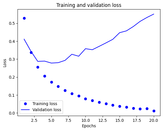
  

  複製

  

  • 繪製訓練和驗證準確度

  plt.clf()
  acc = history_dict['accuracy']
  val_acc = history_dict['val_accuracy']
  
  plt.plot(epochs, acc, 'bo', label='Training accuracy')
  plt.plot(epochs, val_acc, 'b', label='Validation accuracy')
  plt.title('Training and validation accuracy')
  plt.xlabel('Epochs')
  plt.ylabel('Accuracy')
  plt.legend()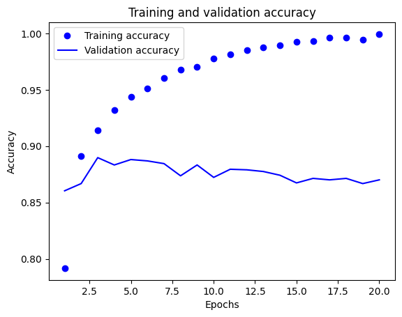
  

  複製

  

  • 從結果可見，訓練集的損失隨訓練週期增加而減少，準確度隨週期增加而增加，但是對驗證集而言，卻沒有得到一樣的成效，這就是 過度配適(overfitting) 的現象。
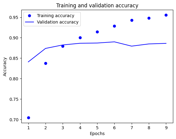
  • 我們可以使用其它技術來避免 overfitting 的發生，如 early stop、drop out

  from tensorflow import keras
  from tensorflow.keras import layers
  from tensorflow.keras.callbacks import EarlyStopping
  
  model = keras.Sequential([
      layers.Dense(16, activation='relu'),
      layers.Dropout(0.5),
      layers.Dense(16, activation='relu'),
      layers.Dropout(0,5),
      layers.Dense(1, activation='sigmoid')
  ])
  
  model.compile(optimizer='rmsprop',
              loss='binary_crossentropy',
              metrics=['accuracy'])
  
  early_stopping = EarlyStopping(
      monitor='val_loss',
      patience=4,  # 連續4個epoch沒改善就停止
      restore_best_weights=True  # 回復最佳權重
  )
  
  x_val = x_train[:10000]
  partial_x_train = x_train[10000:]
  y_val = y_train[:10000]
  partial_y_train = y_train[10000:]
  
  history = model.fit(partial_x_train,
                      partial_y_train,
                      epochs=20,
                      batch_size=512,
                      validation_data=(x_val, y_val),
                      callbacks=[early_stopping])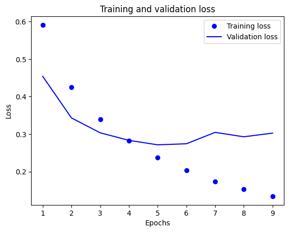
  

  複製

  

  • 拿來測試驗證集

  predictions = model.predict(x_test, batch_size=128)
  test_loss, test_acc = model.evaluate(x_test, y_test)
  print(f'test_acc: {test_acc}')
  
  > test_acc: 0.8849200010299683
  

  複製